Antenna and Network Analyser Basics
What are those S-parameters ... a DUT ... Spectrum, Network Vector or Skalar Analyser?How to use a Network Analyser for measuring Antennas, Coax Relays, Filters and alike ...
Reading a Smith Chart - Mission Impossible?
Measuring Examples
Aim of this website in contrast to many PDFs and writings on skilled Network Theory we find on the internet, is to give an overview on types of analysers the radio amateur might work with. Further to give practical examples how to deal with typical subjects the radio amateur is interested in like plotting home made filters, determining isolation and insertion loss of a coax relay or simply verifying an antennas frequency response.
I might use some not 100 percent correct terminology here in order provide access to this complex topic for the non RF scientifically graded layman. However I absolutely do recommend to have a second look into serious publications on S-parameters and Network Theory to get the wholeshot of this right to any reader, who shows further interest. In the very best of intensions this little read will encourage readers that have spared no effort to get into these complex topics up to now and continue their education with more scientific read.
Preface & Intro
to 'use of VNA & Antenna analyzer in the real life' (www.ok2kkw.comThere are Spectrum Analysers, Antenna Analysers, Vectoriel Analysers, Scalar Analyser, VNAs that are mentioned or advertised for measuring RF parts. But what is the difference? Which Analyser is for what task or what are these types capable to do?
In contrast to an Antenna Analyser a Network Analyser provides two coaxial bushings were you can connect some coax cables. In strict terminology we name these 'ports'.
• Single port: An Antenna Anaylser is a 'real' analyser too. Just with only a single port, because that is what it needs to measure antennas as antennas possess a single port, their terminal.
• Two ports: For Two-port devices like a bandpass filter we need a two-port analyser to measure their characteristic curve.
Spectrum Analyser vs. Network Analyser
• a Spectrum Analyser is passiv - it does not 'TX'. It will not send a signal from its port. Thus it cannot plot any reflections.• a Network Analyser can send a signal from a port and plots the 'answer' received from the Device under Test on same or other port
A Spectrum Analyser is useful for tracing harmonics from a transmitter and things like that. To monitor signal purity of a transmitter. But with it we can not plot passive devices like a filters curve. It can be turned into a Network Analyser by adding a sweep signal generator (Tracking Generator) though. Often Spectrum Analysers are sold as a 'matched pair' together with a fitting tracking generator that suits the Spectrum Analysers frequency span and dynamic range. A Network Analyser simply put is a two-in-One. Signal (ie. Tracking) Generator and Spectrum Analyser in one box.
• Network Analyser = Spectrum Analyser + Tracking Generator
Types of Network Analysers
• a Antenna Analyser is a One-Port Analyser
• a Network Analyser is a Two-Port Analyser
• but there are also vectoriel and non-vectoriel Antenna Analysers
• non Vectoriel Analysers are called Scalar Analsers, they can plot magnitudes only
• non Vectoriel Analysers Network are called Scalar Network Analsers, SNA, they are capable of plotting magnitudes only
• a VNA is a Vectoriel Network Analyser. It is capable of plotting phase ie. imaginary jX too, see here
Antenna Analysers and Two-Port Network Analysers are capable of measuring ratios of power send and reflected. Either from port to port or sent from the single port and reflected amount that runs back to that port. We could say the Antenna Analyser pings the Antenna and listens to a response, ie. reflections of his own signal on the same port. In the Network Theory the 'Two-Port-Network' that our Network Analyser provides with its two coax connections offers a set of parameters that describe what is going on between these two ports (a) and (b). Port (b) is but a clone of port(a). Both can receive and transmit. So we can use a signal path from port (a) via the DUT to port (b) and name these Forward Reflections, and in reverse transmitting from port (b) via the DUT into port (a) and name these Reverse Reflections.
Scatter Parameters - 1
This set of parameters is called S-parameters (Scatter Parameters). The name 'Scatter' rightly deduces what happens in Meteor Scatter or Backscatter radio. Some transmission originating at a point (a) is reflected at an other point (the Device under Test) and received at port (b). Quality and quantity of reception are determind by the grade of the Scatter phenomen. Lets move for this little play of words to another crude analogy. EME. As a rather simplified model a ham station transmits to the moon and listens for its own echos. The signal originates and returns to same port. Quality and Quantity of the received echo are determined by the properties of the Scatter Object - the moon. At least if we skip the immense path loss for a minute.
Who has visited this website?
Antenna Analyser
This is what a One-Port or Antenna Analyser can do.

DUT = Device Under Test
Introducing a to be measured or tested device to port (a) or between ports (a) and (b) equals the meteor trail or moon in our simple RF distribution equivalents. In 'Network Speak' the to be tested or analysed device is named Device under Test = DUT.
The first of these S-params describes what is returned to port (a) from the DUT
S11 = (Input) Reflection Coefficient (s. here for all S-parameters
The Reflection Coefficient mathematically is what commonly known is as VSWR or Return Loss (RL). All three are hold the same information, just in different notations. With the right formula these measures can be converted into the other. Here
Reflection as
Coefficient (numeric)     RL. dB       VSWR
              0.01       (-)40.0       1.02
              0.10       (-)20.0       1.22
              0.20       (-)14.0       1.50
              0.50       (-) 6.0       3.00
              1.00       (-) 0.0     Infinite
YU7EF's EF7017 : simulated VSWR

Network Analyser
A Two-Port or Network Analsyser can do all the Antenna Analsyser does from port (a)
A Two-Port Network Analsyser can tramsmit from port (a) and receive at port (b) and vice versa. Which in our simple model is a QSO via the moon as DUT. Again with path losses skipped.
If we now connect our DUT of choice, lets do a coax relay, to the analyser, the transmission from port (a) can also be received at port (b), a transmission from (b) be received at (a). All with the DUT inbetween. The DUT changes attenuation and phase between the two ports
Transmisson Mode
The influence of the DUT over selected frequency span will also attenuate in the pass (a) -> (b) and (b) -> (a). Which opens up new ways of measuring more of these exciting S-params. Now we can analyse our DUT in 'Transmission Mode' too.
![]()
 Caution must be taken to ensure that the power level at port (b) does not exceed specified maximum level.
Plotting Gain Blocks as LNAs or PAs we need to insert an attenuator. For details see 'Samples' below.

Scatter or S-Parameters - 2
A set of four S-params fully describes what is going on either side the Two-Port Network:

|
For Port (a) that are S11 = Forward (Input) Reflection Coefficient S21 = Forward Transmission Gain* from Port (a) to Port (b) For Port (b) that are S12 = Reverse Transmission Gain* from Port (b) to Port (a) S22 = Reverse or Output Reflection Coefficient |
Mind that 'gain' must be seen in an abstract sense here ... loss as attenuation is gain into minus direction. An ordinary -10 dB attenuator is a -10 dB gain block. A car breaking is described by physicists as negative acceleration. The Transmission Gain params S21 and S12 measure the attenuation of likewise a filter as DUT as 'minus gain', for an LNA put between the ports that is 'positive gain' then. Mind inserting an attenuator of same number as the amplification gain of the LNA behind the amplifier the LNA ... not to crack the analysers port input circuit (!)
The following images (1-7) are screenshots made from the electromagnetic (EM) RF circuit simulation tool
Sonnet EM Lite (TM) by Sonnet Software Inc. ⁄ DUT is a 432 MHz 5 pole QRO Low Pass Filter (LPF)
→ Place mouse over images to enlarge

 |

 |
|
|
(1) Advanced circuit simulation programs make use of S-Params: Plot menu of Sonnet EM Lite (TM) by Sonnet Software Inc. • Note options 'Magnitude (dB)' or • 'Magnitude' = numeric = as coefficient |
(2) A 432 MHz Low Pass Filter plotted as S11 param : Input Reflection with Magnitude in dB. 'Deep' Reflection in minus dB is good VSWR to the layman. The filters RL at 0.43 GHz is better -35 dB or VSWR 1.04 or 0.018 numeric coefficient |
→ Place mouse over images to enlarge

 |

 |
|
|
(3) Same with S21 param : Forward Transmission Gain (red) in dB from port (a) to (b) - what the PA 'sees' - added to x-axis on right side S21 and the reverse S12 param are the 'classical' filter attenuation curves. |
(4) Same with S12 param : Reverse Transmission Gain (red) from other port (b) to port (a) - that would be the antenna side. There is not much of a difference to the S21 param here. The LPF is quite symmetrical. |
→ Place mouse over images to enlarge

 |

 |
|
|
(5) Same with S22 param : Reverse Reflection (red) with Magnitude in dB (That would be filter Return Loss or VSWR looking from antenna side) The good filter it is, both Reflection curves S11 and S22 are very close, so we see a 99 percent overlay of both curves. |
(6) And S11 param : Input Reflection as coefficient (numeric) and plotted as Smith Chart. We find best = lowest attenuation close to the wanted 432 MHz; with a numeric magnitude close to zero (VSWR = 1.06). |
→ Place mouse over images to enlarge

 |
||
|
(7) Same LPF plotted with Z_in as param : Input Impedance in ohms on right side x-axis |
And suddenly all those notations hopefully do make sense.
Another example:
A coax relays port isolation to the not switched to connector. This is the 'gain' as attenuation of the transmisson at port (a) through the coax relay as DUT - 'listened at' and measured at port (b). S21 param 'Transmission Gain' is pretty lossy here.
S21 param : Forward Transmisson Gain : A Coax Relays Port Isolation, sweep range 50 to 1300 MHz
More Theory
Numeric Gain? Reflection Coefficient??
We are used to find gain and loss given in dB. But the 'natural' way for S-params and many calculations is
to give and handle gain etc as numeric factors. Using maths log and exp functions we can transform form the
log. scaled measure Decibel to its numeric value.
I am explaining this because most analysers can display the set of S-params in either notation.
So you opt for S11 or whatever other in dB in your analysers setup or menu for any ham related 'standard' measurement.
dB Conversion Calculator
This conversion works with GAIN and LOSSES:
• Gain 3.0 dB = 2.00 numeric
• Gain 0 dB = 1.00 numeric
• Gain -3.0 dB = 0.50 numeric
But how do we deal with coax line losses from and to our DUT?
We do this in three steps. First measure the complete 'circuit' consiting of measurement line from port (a) to DUT, the DUT itself and measurment line back to port (b) of the analyser. In a second step we replace the DUT by a quality adapter between the ends of both measurement lines. This way we can plot the behaviour of our lines solely. Which we then subtract from the attenuation at cutfoff or corner frequencys of that fiter as DUT.
Task: DUT is a commercially made Coaxial Stepped Impedance 470 MHz Low Pass Filter. How to measure what attenuation will it provide if we use it in line with our PA on 432 MHz?
Step 1: Measuring the filter using the S21 parameter or Transmisson Mode
![]()
made Coaxial Stepped Impedance 470 MHz Low Pass Filter. What attenuation will it provide if we use it in line with our PA on 432 MHz?
Step 2: the DUT removed and open measurement lines connected with a quality female / female N instead
Place markers on same frequencies of interest as in DUT plot for comparsion and subtracting numbers in step 3.

Which is 1.827 dB - 1.530 dB = 0.297 dB.
Note the response of the attenuation over increasing frequency from 0.2 to 1.3 GHz. The lines are 2 x 2.7 m of RG-142
PTFE coax surplus with quality N-connectors.
THE OTHER WAY of dealing with losses and phase shifts the connection lines bring with them ...
is to calibrate the analyser on these. But then we need to repeat the calibration routine whenever we are using an other coax to connect a DUT. Furthermore a calibration on a single frequency will do for measurment sweeps in close range around that frequency. But for the shown coax relay plots over a span of 50 ... 1300 MHz a realistic adaption of measurement line losses is not practicabel with such. Unless the analyser is capable of running a sweep calibration and storing the whole range of losses and phase shifts over a given frequency span.
Analyser Calibration
Actually a quality analyser deserves a quality calibration kit because it can hardly be more accurate then the source of calibration. Hmm ..? Another topic: Analyser calibration
With our 3 Step method to do a baseline plot of the circuit whit DUT excluded we can not go wrong but for the absolute calibration to 50 ohms and zero gain. But any measurement tool needs to be calibrated and probably be recalibrated from time to time. If the base calibration is bad we hit bad ground with whatever we measure, though the baseline method decreases the offset to linearity of magnitude challenges only.
An analyser calibration kit usually holds
• a short piece of coax to short circuit between ports (a) and (b) to null param gain
• a precision termination load to null params R and jX
• optionally one or more precison attenuators and or phase shifting test DUTs for comparing and testing an numbers
Alright, commerical quality calibration kits are expensive precision items. For any 'household quality' measurments up to the 2 m band we can produce a private calibration kit ourself. A shortes, best quaility coax with also best quality connectors may serve as the short circuit coax. A low power terminator with least jX, like a 3 GHz capable load may be good enough to calibrate Z for 144 MHz. Ideally we have a friend who can do use a reference on our own kit with a high standard analyser.
What else?
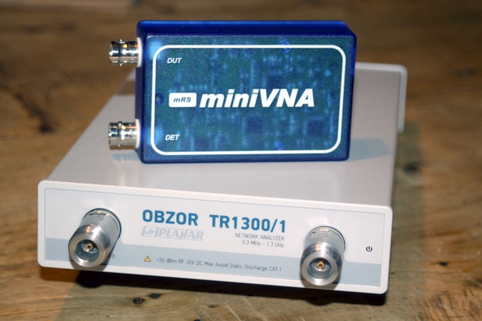
With any 'cheap' analyser or whenever in doubt or from time to time (calibration intervals ... for whatever measurement device) we might check its frequency scale. In case not frequency counter is at hand we can use our TRX for this. I can pick up likewise my miniVNA's sweeps turnpoints as cracking noises. For this I have the VNA doing a sweep form 144.100 to 144.500 or whatever and listen on 144.200 having my Yagi on the roof connected. An easy and cheap method.
Scalar or Vectoriel Analyser?
All of the shown above examples can be executed with a scalar analyser. Since we have not looked at phase shifts respectively imaginary components of the impedance of our DUT yet. When we are looking a attenuation or gain only the match to the impedance of our analsysers ports is included. We better say - the matching losses to the ports impedance are included .. automatically.
But if we want to know what is really going on in terms of a good match to 50 ohms likewise for an antenna feedpoint or self designed and build filters we will have to know WHAT actual impedance the two ports of our DUT has and HOW that is composed. Meaning what imaginary part it may hold.
The scalar analyser (just) measures numbers on a scale, like insortion loss over frequency
The vectoriel analyser additionally can measure the phase angle between real and imaginary component of a signal. The name giving is due to a vector starting at zero-point of the coordinate system describing the complex number plane. The vectors lenght describes 'strength' or attenuation or gain, its orientation is given in the phase angle. Which then holds the imaginary amount. Which is X as capacitve or inductive part of the impedance.
Impedance: Z = R + jX
If you resign at the sight of a Smith Chart ... look up the sections below in which the Complex Numbers Plane and Smith Chart are explained in simple words.
S11 param : Forward Reflection : vectoriel : plotted into a Smith Chart
Complex Plane - Mathematical munition for reading a Smith Chart in a Nutshell
• Step 1: The complex number plane in mathematical universal notation
Reading a Smith Chart - Mission Impossible?
Once we have taken that the vector z or Z for impedance is characterised by length (Z) and phase angle we note that the display in a complex plane is a screenshot on a single frequency only. A filter as combination of a number of inductances and capacitances shifts the phase angle in every component. That is what coils and capacitors do in a mathemactical description of their properties refering to an applied frequency.
The Smith Chart now shows the movement of the phase angle and thus the vector over a frequency span. But how?
Let us develop the Smith Chart by ourselfs.
We want to show R and jX over frequency. So we introduce a frequency axis were the Real Part has been on x-axis of the Complex Plane. Now what to do with the former Real (Re) axis? For this parameter we define stretches in the new chart which define the Real Parts, our R (the diagonal grey lines). Now we can place a dot = x(Freq, R, jX) according all three parameters
• Frequency
• Real Part : R
• Imaginary Part : jX
A completely simplified sketch of the idea of how the Smith Chart works

• The light blue curved lines are of same jX
• The grey circles are lines of same R in ohms.
The example shows likewise a 70 cm Yagi-Udas feedpoint impedance above band end.
The higher the R, the closer to the right were the circles touch we go.
The higher the jX, the more we move out of the mid frequency line, upwards for inductances, down for capactiances.
Samples
Measuring Resonace Frequency of a Coax Stub
with a Vectoriel Network Analyser
A Network Analyser can perform S21 or Transmission Mode. So it plots the gain or attenuation of a signal send at port (a) and received at port (b) over the chosen frequency scan range.
Principle (Port a) = DUT and (Port b) = DET:
What is going on here? How does this work?
This image shows a screenshot done with the popular miniVNA whose menu names S21 as Transmission Mode. Being a Vectoriel Analyser it can display the Phase(shift) the DUT applies on the path from port (a) to port (b). The DUT now consists of the coupling between the shown small coils plus the introduced interference in form of the stub. The stub, being resonate as a quarter wave circuit line (and harmonics) will significatly shift the phase in our constructed path at any frequency of resonance.
miniVNA plot of stub: Transmisson Mode (T.L.) on right gain / loss in dB, note Phase in degr. as parameter on left.
We are not after a specific phase or form of the spike here. All we want is to find out were the spike is going to occure
Same as S21 parameter: A piece of H2010 trimmed to resonate at 144.1 and harmonics (with OBZOR / Planar TR1300 VNA).
Scan sweep range is 40 to 1000 MHz to show a number of harmonics too


Combiners / Splitters
Doing a quaility plot on splitters requires quality terminations on all open splitters ports (!). These shall be of same make and connected with least number of whatever adapters or coax cable. An ideal plot only works wiith directly connected, small terminators ... as every bit of extra length virtually adds to the 1/4 λ or 1/2 λ length of the splitter. If you do not have the needed number of good loads, sorry to be frank here, but forget about a quality plot of your splitter.
(Side note: As so often when about to craft something technical of quality it needs tools and measurement equipment to get there. Think of the money you may save and the joy you may find in producing a home meade device with high quality instead of buying a splitter and spend some money on termination loads now you have spend much more on the analyser itself. These splitter mesurements only get as precise as the provided loads are in both, total Z and amount of jX.)
Here is how it is done:
The photo shows a 432 MHz Quarterwave Splitter, four similar, high spec. and directly connected termination loads, an miniVNA - pro with added extender (a capable combo for the job)

And what do we get in return?
S21 param : Forward Transmission gain plotted in dB - scale and phase for controlling the frequency response (fig. 1)
and Z respectively VSWR for controlling input impedance (fig. 2)
Fig. 1: Plot of a 1/4 λ 4 x splitter for 144 MHz / 'RP' is Phase in the miniVNA-pro's operating software

See what parameter Phase (light blue line / 'RP') does in the plot above?
It yet again changes sides, exactly at point of resonace.
Fig. 1: Plot of a 1/2 λ 4 x splitter for 144 MHz

And what about measuring the other splitter ports then?
If the above plots of S21 and Z give the wanted result there is no need to do the other ports, provided we have terminated them with quality loads. Because if so, the splitter must work. The four termination Z's against the splitter transformation ratio at designated frequency can not deliver anything apart from the exact ratio provided the loads are of sufficient specification and all equal.
These Splitters have been build according my Coax & Splitter Calc. website, see here for more
Gain Blocks
For measuring Gain Blocks (vulgo : Amplifiers) with a Network Analyser we need to introduce an attenuator to our line circuit. Because the receiving ports of an analyser are made for power levels same as the tramsitting ports. Which depends on the model but surely is in the 'few' milliwatt range or even lower. The important lesson is that you must not feed a signal orginated at one port and amplified by 10, 20 or 40 dB into the other port. Or even worse, expose any analyser port to power from a 'real' power amplifier.
Caution must be taken to ensure that the power level at port (b) does notexceed specified maximum level. Otherwise the Analsyser might be damaged!
Take care, use appropriate attenuators, use higher attenuation when ever the gain to
be expected is unknown yet. Think of a test build of a preamplifier that suddenly
starts to oscillate. You can easily use like 20 dB higher attenuation to start with.
Then take a frist plot and adjust your attenuation level upon that result.
But: be sure to sweep a large enough frequency range to detect oscillationsin the microwave region OR use a low pass filter in line with the attenuators to
be on the safe side here!


Which does not prevent us from measuring that amplifier.
As shown how to deal with the coax line losses we can use any higher attenuation block and reverse calculate the amplification gain refering to that number.
• (1) Practically we can do a short circuit sweep in S21 param : Forward Transmission Gain
• (2) Do a baseline measurement of the coax lines, adapters and whatever is enclosed plus attenuator over sweep range
• (3) Place markers at frequencies of interest like 420, 430, 432, 440 and 450 MHz for a 70 cm LNA
• (4) read out numbers or do a screenshot
• (5) Next mount the LNA as DUT and do a sweep.
• (5) Finally subtract the baseline dBs ie. losses at those frequencies of interest
... and have a fine view on the real gain per frequency of this amplifier.
Further read for the ambitioned RF technician:
Link to www.keysight.com, Presentation 'Basics of RF Amplifier Test with Vector Network Analyser (VNA)' by Taku Hirato, Agilent Technologies Inc.
as PDF

This large presentation needs some time to load
... to be continued
73, Hartmut, DG7YBN